
Improving Forecasting of High-Demand Weekly Data
High Demand Weekly Data Forecasting
The Business Problem
QueBIT clients have traditionally asked for forecasts derived from historical monthly demand data. While monthly forecasts can still be very helpful, increasingly sophisticated data collection procedures have allowed clients to start providing QueBIT with data at the daily or weekly level.
A consequence of granular data like daily or weekly is that there is simply more data for our models to be trained on, which can potentially reveal seasonal patterns (e.g.,with daily data you may see more sales on Friday than Monday, though seasonality with weekly data is a little more tricky) that are obscured at the monthly level. In turn, demand planning can proceed with increased precision if a client requires it.
In this notebook, we will work with a standardized set of data at the weekly level and see if we can improve forecasting performance over QueBIT’s previous method.
Setup
First I began with loading the libraries I expected to need for this project and set the random seed so that the results are reproducible.
# Change settings to not use scientific notation
options(scipen = 999)

# Set random seed
set.seed(401)

# Load packages
# Data manipulation.
library(tidyverse)
library(data.table)
library(here)
library(lubridate)
library(future)
library(reticulate)
library(kableExtra)
library(tsbox)
library(magrittr)

# Plots
library(ggplot2)
library(patchwork)

# Analyses
library(fable)
library(fabletools)
library(feasts)
library(tsibble)
library(fable.prophet)

# Set plot themes
theme_set(theme_bw())
Next I set the working directory:
# Set working directory based upon location of this notebook
i_am("WeeklyHighDemandData.Rmd")
I then cleaned the data, first by rolling it up to the weekly level from the daily level (the daily level contains many days with zero demand, which will create problems for statistical forecasting models).
# Read in data
df <- fread(file="WeeklyHighDemand.csv") %>%
  select(-7:-12) %>%
  as_tibble()

# Create weekly dataframe from daily data
df_weekly <- df %>%
  group_by(sku, date = yearweek(transaction_date)) %>%
  summarise(gross_units=sum(gross_units,na.rm=TRUE))

# Convert to tsibble (time series tibble) with SKU as key
df.ts <- df_weekly %>%
  as_tsibble(index=date,key=sku)
This data set contains many SKU’s where there is simply insufficient historical data for forecasting:
# Count # of rows of data for each SKU
counts <- df.ts %>%
  as_tibble() %>%
  count(sku) %>%
  arrange(desc(n))

# Get descriptives of the number of rows per SKU
kable(counts %>%
  summarise(median=median(n),
            mean=round(mean(n),digits=2),
            min=min(n),
            max=max(n))) %>%
  kable_styling()
| median | mean | min | max |
|---|---|---|---|
| 35 | 56.38 | 1 | 187 |
# Filter to only those combos with the maximum of 187 weeks
df.ts %<>%
  group_by(sku) %>%
  filter(n()==187)
For ease of presentation, I filtered the data just to the SKU’s with 187 weeks of historical data (the maximum in the dataset). This leaves 698 SKU’s in the dataset for analysis.
Another innovation that I added to forecasting pipeline is the use of something called the Ljung-Box Test. This test checks whether a SKU has enough predictability in its historical data (“autocorrelation”). A lack of predictability means that the time-series is “white noise” and is therefore unpredictable by statistical models (but may be good candidates for neural network approaches that don’t rely on autocorrelation).
# Perform Ljung-Box test
lb <- df.ts %>%
  as_tibble() %>%
  group_by(sku) %>%
  summarise(test=ljung_box(gross_units,lag=52)[2])

# How many of the time-series are white noise?
lb %<>%
  filter(test < 0.05) # 446 SKU's are not white noise

# Filter main dataset down to those that are not white noise
df.ts %<>%
  filter(sku %in% lb$sku)

# Remove large data frames to free up memory
rm(df,df_weekly)
446 SKU’s survived the Ljung-Box test and will be used in our competition to determine which models work best for this data.
Fitting new forecasting models
I next fit 7 different statistical models to the data, ranging from very simple models like using the grand mean to predict the test data, all the way to modern methods like Meta’s Prophet algorithm. Each model was fit to each SKU in an iterative fashion. I first split the data into training and testing sets using an 80/20 ratio.
The models were then fit to the training data and combinations forecasts, which take the predictions from several models and average them together, were calculated. This was another feature that was not available in QueBIT’s previous forecasting approach that was added at my suggestion. Finally, forecasts were performed on the held-out testing set and accuracy was calculated using MASE scores (a measure of mean absolute error relative to the performance of the naive model for that SKU, MASE scores under 1.0 mean that the model outperformed a Naive approach).
# Create training set using data 80% of the data
train <- df.ts %>%
  group_by(sku) %>%
  slice_head(prop=0.8) %>%
  as_tsibble(key=sku,index=date)

# Create testing set with remaining 20%
test <- df.ts %>%
  group_by(sku) %>%
  anti_join(train)

# Define decomposition model (Old QueBIT approach)
STLF <- decomposition_model(
    STL(gross_units),
    ETS(season_adjust)
  )

# Fit models to the training data
plan(multisession) # use all cores available on CPU

test.models.weekly <- progressr::with_progress(train %>%
  model(
    Mean = MEAN(gross_units),
    Theta = THETA(gross_units),
    ETS = ETS(gross_units),
    Linear.Regression = TSLM(gross_units),
    ARIMA = ARIMA(gross_units),
    QueBIT_Old = STLF,
    Prophet = prophet(gross_units ~ season(period="year",3))) %>%
  mutate(Intermediate.Ensemble = (Theta + Linear.Regression + ETS +
                                    ARIMA + QueBIT_Old)/5,
         Kitchen.Sink.Ensemble = (Mean + Theta + Linear.Regression +
                                    ETS + ARIMA + QueBIT_Old + Prophet)/7))

# Forecast testing data
plan(multisession)

fc.test.weekly <- test.models.weekly %>%
  forecast(test)

# Check accuracy of the forecasts
test.acc.weekly <- fabletools::accuracy(fc.test.weekly,df.ts)
Accuracy of new models
Because each SKU had 7 different models fit to it, one model may be better for that particular SKU than other models. So I first determined which model was the most accurate for each SKU, and then aggregated the number of SKU’s for which each model was the top performer. This allows us to take into account the possibility that one model may have achieved excellent accuracy, but only for a few SKU’s, which makes the relative value of that model overall somewhat questionable.
# Calculate best fitting models
best.test.weekly <- test.acc.weekly %>%
  group_by(factor(sku)) %>%
  filter(MASE==min(MASE))

lowest.mase.weekly <- best.test.weekly %>%
  group_by(.model) %>%
  summarize(n=n(),
            avg.MASE=mean(MASE)) %>%
  arrange(-n)

kable(lowest.mase.weekly,
      col.names = c('Model', 'Num. of SKUs it was best for', 'Average MASE'),
      caption = "Average MASE score by model on weekly high-demand data",
      digits = 3) %>%
  kable_styling(bootstrap_options = "striped",
                full_width = F,
                font_size = 18)
| Model | Num. of SKUs it was best for | Average MASE |
|---|---|---|
| Theta | 93 | 0.558 |
| Prophet | 73 | 0.750 |
| Kitchen.Sink.Ensemble | 68 | 0.616 |
| ETS | 52 | 0.578 |
| Intermediate.Ensemble | 52 | 0.608 |
| ARIMA | 46 | 0.640 |
| Linear.Regression | 25 | 0.857 |
| Mean | 25 | 0.852 |
| QueBIT_Old | 22 | 0.885 |
Looking at the table above, we can see that the Theta model was a strong performed for the largest number of SKU’s. Two more new additions, the averaged forecast of all of the forecasts (Kitchen.Sink.Ensemble) and Meta’s Prophet also performed well for a large number of SKU’s. Perhaps most importantly, we vastly improved accuracy over QueBIT’s old method of forecasting, which was the top performing model for only 22 SKU’s out of 446.
Improvement in accuracy over old QueBIT forecasting approach
What is most important is how much these new models were able to improve forecasting accuracy over QueBIT’s old forecasting pipeline. I filtered down to the SKU’s for whom any model other than QueBIT’s old approach was the best performing. I then took the accuracy of QueBIT’s old approach for that SKU, and compared it to the best performing model on that SKU.
# Create a dataframe with SKU's where old QueBIT approach was NOT the best
quebit.not.best <- best.test.weekly %>%
  group_by(sku) %>%
  filter(.model!="QueBIT_Old") %>%
  distinct(sku,.keep_all=T) %>%
  ungroup()

# Get the accuracy of the old QueBIT approach on those SKU's
quebit.old.performance <- test.acc.weekly %>%
  filter(sku %in% quebit.not.best$sku) %>%
  filter(.model=="QueBIT_Old")

# Join tables together and calculate % improvement for new approach
new.improvement <- quebit.not.best %>%
  full_join(quebit.old.performance) %>%
  group_by(sku) %>%
  summarise(pct.improvement=1-(min(MASE)/max(MASE))) %>%
  mutate(pct.improvement=round(pct.improvement*100,2))

# Create plot data and then plot comparison
plot_data <- full_join(quebit.old.performance,quebit.not.best) %>%
  mutate(x_label=ifelse(.model=="QueBIT_Old","QueBIT old approach","Best fitting new model"))

ggplot(plot_data,aes(x_label,y=MASE)) +
  geom_boxplot() +
  geom_hline(yintercept=1,linetype="dashed") +
  stat_summary(fun="mean",shape=4,size=1,color="red") +
  ylab("MASE Score (lower is better)") +
  ggeasy::easy_remove_x_axis("title") +
  ggeasy::easy_text_size(16) +
  ggtitle("Improvement by new models over old approach")
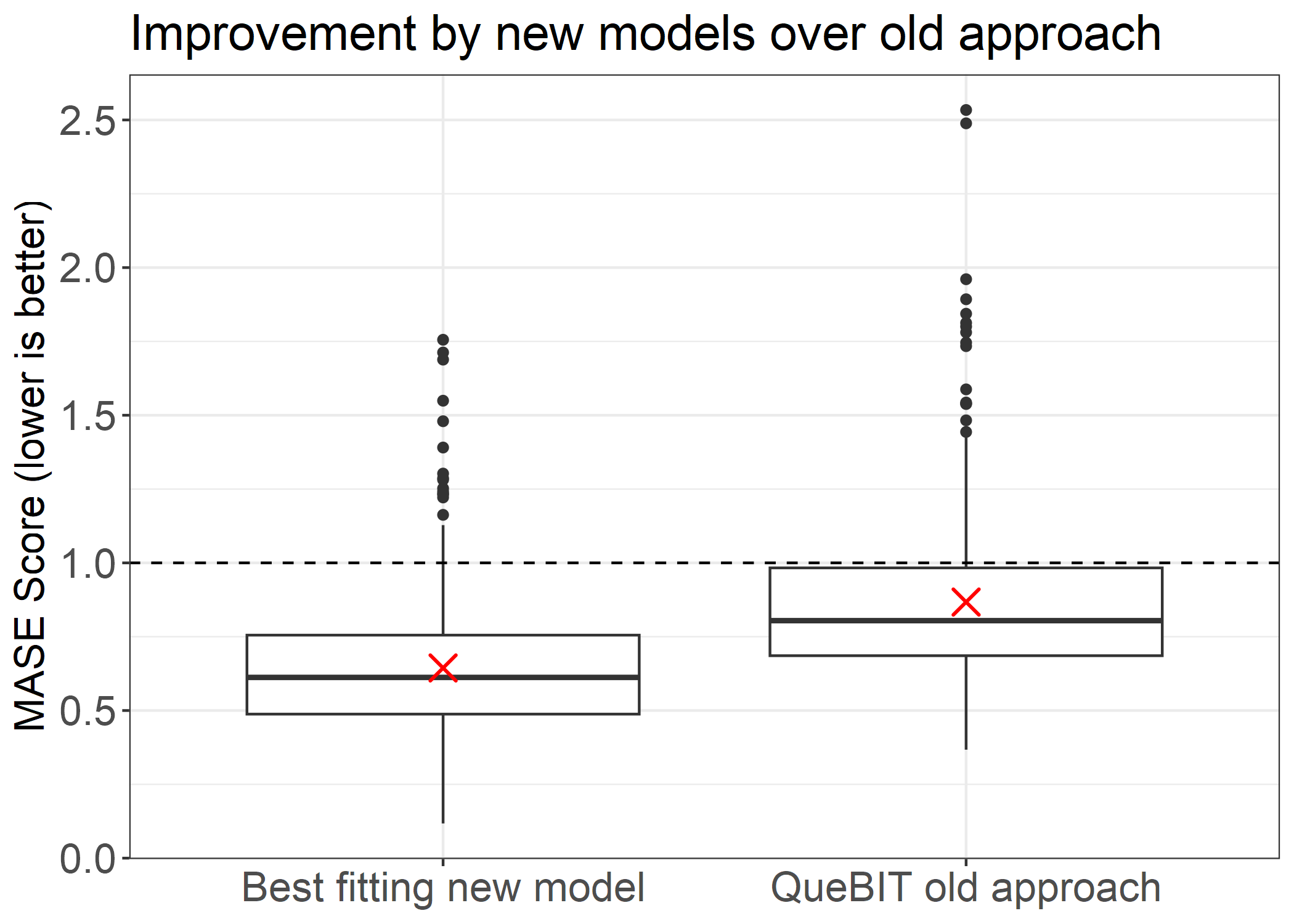
The average percent improvement was a whopping 25.56 % increase in accuracy. That means that for 424 out of 446 SKU’s, my new approach improved forecast accuracy by an average of 25.56% over the old approach that QueBIT took.