
Using Hybrid Deep Learning/Statistical Model for Forecasting
The Business Problem
QueBIT often has clients who require forecasts of products whose sales are sporadic and may not follow any obvious seasonal patterns. This presents a difficult situation for QueBIT consultants, who may not be able to provide satisfactory forecast for a client, as statistical forecasting models, like ARIMA, generally will not outperform a naive forecast (taking the previous periods’ sales and using it as a forecast for the upcoming period).
Neural networks seem like a viable solution to this problem, as they can handle complex, non-linear relationships that may be overlooked by traditional statistical forecasting methods. However, they have not proven to be a silver-bullet solution for difficult to forecast products - what instead appears to be an optimal solution are methods that combine aspects of statistical forecasting methods and deep learning neural networks, as these “hybrid” approaches have proven their worth in forecasting competitions.
This project serves as a proof-of-concept for the implementation of two hybrid statistical/deep learning forecasting methods for QueBIT, using actual (anonymized) client data. It also is a demonstration of the R Tidymodels ecosystem, which is allows for machine learning analyses within an easily readable and reproducible Tidyverse framework.
Preprocessing of data
This dataset is the same one as in my portfolio project “Improving forecasting on weekly high demand data”, and follows the same steps to preprocess the data. For a more detailed explanation of how I cleaned the data, please see that portfolio. In brief, I first aggregated this data from the daily level (where it was very sparse) to the weekly level. I then limited it to SKU’s that had the maximum 187 weeks of data available. I also removed any SKU’s whose time-series were “white noise” and therefore random.
# Read in data
df <- data.table::fread(file="WeeklyHighDemand.csv") %>%
  select(-7:-12) %>%
  mutate(sku=as.factor(sku),
         transaction_date=as.Date(transaction_date)) %>%
  as_tibble()

# Create weekly dataframe from daily data
df_weekly <- df %>%
  group_by(sku,date=yearweek(transaction_date)) %>%
  summarise(gross_units=sum(gross_units,na.rm=TRUE))

# Filter to only those combos with the maximum of 187 weeks
df_weekly %<>%
  group_by(sku) %>%
  filter(n()==187)

# Perform Ljung-Box test
lb <- df_weekly %>%
  group_by(sku) %>%
  summarise(test=ljung_box(gross_units,lag=52)[2])

# How many of the time-series are white noise?
lb %<>%
  filter(test < 0.05) # 446 SKU's are not white noise

# Filter main dataset down to those that are not white noise
df_weekly %<>%
  group_by(sku) %>%
  filter(sku %in% lb$sku)

# Convert date vector back to base R "date" type
df_weekly %<>%
  mutate(date=as.Date(date)) %>%
  ungroup()

# Remove large data frames to free up memory
rm(df,df.ts)
I first split the data roughly 80/20 into training and test sets, and as a sanity check plotted the data split:
# Split data into training/test
FORECAST_HORIZON <- 37 # 20% of total weeks

# Split training and test
splits <- time_series_split(df_weekly,
                            assess=FORECAST_HORIZON,
                            cumulative=T)
# Plot split
splits %>%
  tk_time_series_cv_plan() %>%
  plot_time_series_cv_plan(.date_var = date,
                           .value=gross_units,
                           .interactive=F)

Next I begin the process of feature engineering, which is the process of transforming the data to make it ready for a neural network. These hybrid approaches are implemented in such a way that they can be given a vector with dates, unlike a conventional neural network, but I chose to engineer more vectors from that date column to potentially improve performance. Tidymodels outputs a neat summary of the feature engineering steps added to a recipe, which can be seen below:
# Create recipe for feature engineering deep learning models
# Step 1. Create timeseries features from date column
# Step 2. Remove some nonsensical vectors, like those for the minute/hour of the day (more granular than original data)
# Step 3. One-Hot encode any non-numeric variable (like month name)
# Step 4. Remove zero-variance features

recipe_spec_deeplearning <- recipe(gross_units ~ .,
                                   data = df_weekly) %>%
  step_timeseries_signature(date) %>%
  step_rm(contains("iso"), contains("minute"), contains("hour"),
            contains("am.pm"), contains("xts")) %>%
  step_dummy(all_ordered_predictors(), one_hot = TRUE) %>%
  step_zv(all_predictors())

# Prep recipe (gives overview of what will be applied to training data)
prep(recipe_spec_deeplearning)
##

## ── Recipe ──────────────────────────────────────────────────────────────────────

##

## ── Inputs

## Number of variables by role

## outcome:   1
## predictor: 2

##

## ── Training information

## Training data contained 83402 data points and no incomplete rows.

##

## ── Operations

## • Timeseries signature features from: date | Trained

## • Variables removed: date_year.iso, date_week.iso, date_minute, ... | Trained

## • Dummy variables from: date_month.lbl, date_wday.lbl | Trained

## • Zero variance filter removed: date_second, date_wday, ... | Trained
Fitting N-BEATS and DeepAR models
With our recipe in place, we can now start creating the model specifications for our deep learning models and the statistical models we will compare them to. I am largely using default settings for these deep learning models, and am keeping the epochs low as epoch loss seems to plateau quickly. I used MASE (mean absolute scaled error) as the loss function
# Create model specifications for N-BEATS model
model_spec_nbeats <- nbeats(
  id                    = "sku",
  freq                  = "W",
  prediction_length     = FORECAST_HORIZON,
  epochs                = 10,
  scale                 = T,
  loss_function         = "MASE",
) %>%
  set_engine("gluonts_nbeats")

# Create model specifications for DeepAR model
model_spec_deepAR <- deep_ar(
  id                    = "sku",
  freq                  = "W",
  prediction_length     = FORECAST_HORIZON,
  epochs                = 10,
  scale                 = T,
) %>%
  set_engine("gluonts_deepar")

# Create model specifications for N-BEATS ensemble model
model_spec_nbeats_ensemble <- nbeats(
  id                    = "sku",
  freq                  = "W",
  prediction_length     = FORECAST_HORIZON,
  epochs                = 10,
  scale                 = T,
  loss_function         = "MASE"
) %>%
  set_engine("gluonts_nbeats_ensemble")

# Create model specifications for feed-forward NN with autogression
model_spec_nnetar <- nnetar_reg(hidden_units = 5
) %>%
  set_engine("nnetar", MaxNWts=5000) # need to increase the max number of weights
Instead of just running the deep learning models, I added them to a “workflow”, which is a modular pipeline where different parts of the workflow can be modified without having to remake the model from scratch.
# Create workflow for N-BEATS model
workflow_nbeats <- workflow() %>%
  add_recipe(recipe_spec_deeplearning) %>%
  add_model(model_spec_nbeats)

# Create workflow for DeepAR model
workflow_deepAR <- workflow() %>%
  add_recipe(recipe_spec_deeplearning) %>%
  add_model(model_spec_deepAR)

# Create workflow for N-BEATS Ensemble model
workflow_nbeats_ensemble <- workflow() %>%
  add_recipe(recipe_spec_deeplearning) %>%
  add_model(model_spec_nbeats_ensemble)

# Create workflow for feed-forward NN
workflow_nnetar <- workflow() %>%
  add_recipe(recipe_spec_deeplearning) %>%
  add_model(model_spec_nnetar)
Finally, I fit the deep learning models alongside some statistical models to serve as a comparison.
# Fit N-BEATS model
parallel_start(16)
model_fit_nbeats <- workflow_nbeats %>%
  fit(data=training(splits))

# Fit DeepAR model
model_fit_deepAR <- workflow_deepAR %>%
  fit(data=training(splits))

# Fit N-BEATS Ensemble model
model_fit_nbeats_ensemble <- workflow_nbeats_ensemble %>%
  fit(data=training(splits))

# Fit feed-forward NN model
model_fit_nnetar <- workflow_nnetar %>%
  fit(data=training(splits))

# Fit Prophet model
model_fit_prophet <- prophet_reg(seasonality_daily = F) %>%
  set_engine("prophet") %>%
  fit(gross_units ~ date, training(splits))

# Fit ARIMA model
model_fit_ARIMA <- arima_reg() %>%
  set_engine("auto_arima") %>%
  fit(gross_units ~ date, training(splits))

# Fit ETS model
model_fit_ETS <- exp_smoothing() %>%
  set_engine("ets") %>%
  fit(gross_units ~ date, training(splits))

# Fit Theta model
model_fit_theta <- exp_smoothing() %>%
  set_engine("theta") %>%
  fit(gross_units ~ date, training(splits))

# Model fit TBATS
model_fit_TBATS <- seasonal_reg() %>%
  set_engine("tbats") %>%
  fit(gross_units ~ date, training(splits))

# Model fit Linear Regression
model_fit_lingreg <- linear_reg() %>%
  set_engine("lm") %>%
  fit(gross_units ~ date, training(splits))

parallel_stop()
Now that all of the models are fit, we can present them with the held-out testing data to evaluate their performance:
# Add all fitted models to a table so that operations can be performed on all models at once
models_tbl <- modeltime_table(
    model_fit_nbeats,
    model_fit_deepAR,
    model_fit_nbeats_ensemble,
    model_fit_nnetar,
    model_fit_prophet,
    model_fit_ARIMA,s
    model_fit_ETS,
    model_fit_theta,
    model_fit_TBATS,
    model_fit_lingreg
)

# Calculate accuracy of models on testing data
calibration_tbl <- models_tbl %>%
    modeltime_calibrate(
        new_data = testing(splits),
        id = "sku")
Calculating Accuracy
I filtered the accuracy output to just the best fitting model per combo, and then created a table showing the model name, the average MASE score, and the number of combos for which it was the best model.
| Model | Num. of SKUs it was best for | Average MASE | Median MASE |
|---|---|---|---|
| DEEPAR | 194 | 0.8127578 | 0.7808250 |
| Feed For. NN | 64 | 0.8420053 | 0.7839065 |
| NBEATS ENSEMBLE | 55 | 0.8502815 | 0.8122568 |
| TBATS | 36 | 0.8382943 | 0.7642848 |
| NBEATS | 31 | 0.9703480 | 0.8980330 |
| Linear Regression | 30 | 0.9781459 | 0.8967145 |
| ETS | 15 | 0.8811495 | 0.8238182 |
| THETA METHOD | 10 | 0.7863031 | 0.7470113 |
| ARIMA | 9 | 0.7873581 | 0.7824942 |
| PROPHET | 2 | 0.9666122 | 0.9666122 |
The story that from the accuracy values of the different models is a complicated one, and demonstrates why it is best for a company to have multiple forecasting approaches available to them. If we look purely at average accuracy, then the ARIMA model is generating the lowest MASE scores. However, it is only able to achieve excellent MASE score for 9 products. By contrast, our hybrid/neural network models (N-BEATS, DeepAR, NNAR, N-BEATS Ensemble) are the best performing model for a much larger share of products, and therefore provide a lot more utility. This concept is better presented visually:
plotdata <- best.mase %>%
  group_by(.model_desc) %>%
  summarize(n=n(),
            avg.MASE=mean(mase),
            med.MASE=median(mase)) %>%
  pivot_longer(cols = avg.MASE:med.MASE,
               names_to="criterion",
               values_to = "value")

ggplot(plotdata,aes(x=reorder(.model_desc, value),y=value,fill=criterion,alpha=n)) +
  geom_bar(stat="summary",position="dodge") +
  geom_hline(yintercept = 1,linetype="dashed") +
  scale_fill_manual("Criterion",labels=c("Average MASE","Median MASE"),values=c("black","orange")) +
  scale_alpha("# of SKU's") +
  ggeasy::easy_rotate_labels(which="x",angle=90) +
  ggeasy::easy_text_size(14) +
  labs(x="Model",y="MASE score (lower is better)")
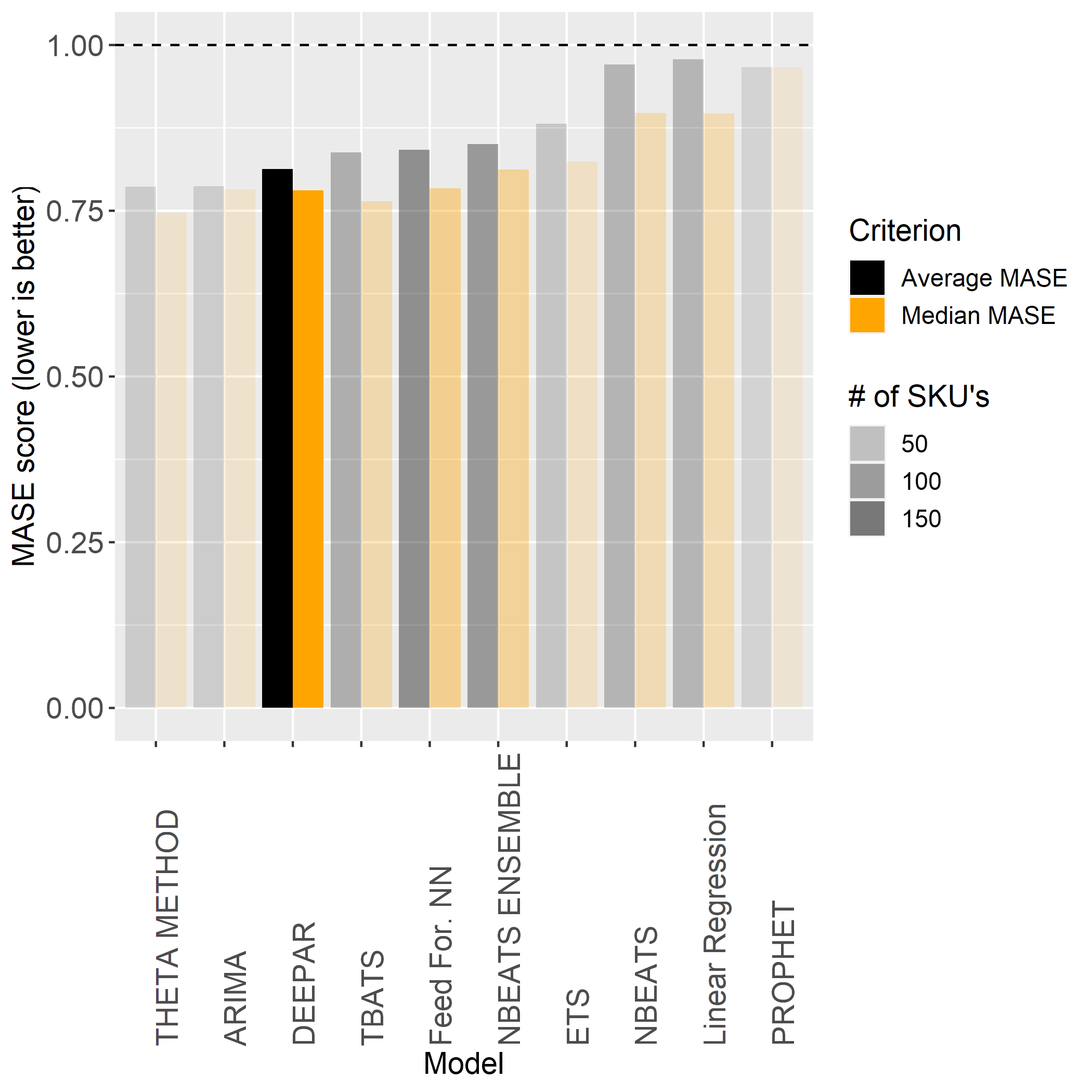
In this plot, we have both the average MASE and median MASE scores shown as bars, and the number of SKU’s it is the best model for is coded by transparency. The DeepAR model is far and away the strongest performer for the largest proportion (43.3%) of the SKU’s in this dataset. It is also a good sign that there is only a relatively small difference between the average MASE score and the median MASE score for the DeepAR models, which indicates that it is consistently performing well across SKU’s and there are few outlier SKU’s that could not be forecast well.
# Calculate scaled MASE scored
best.mase %<>%
  group_by(.model_desc) %>%
  mutate(scaled_mase=scale(mase))

ggplot(best.mase,aes(x=reorder(.model_desc, mase),y=mase,group=.model_desc,size=scaled_mase)) +
  geom_jitter(width=0.20,alpha=0.3) +
  scale_size("Normalized \nMASE score") +
  labs(x="Model",y="MASE score (lower is better)") +
  ggeasy::easy_all_text_size(14) +
  ggeasy::easy_rotate_labels(which="x",angle=90) +
  ggeasy::easy_remove_legend()
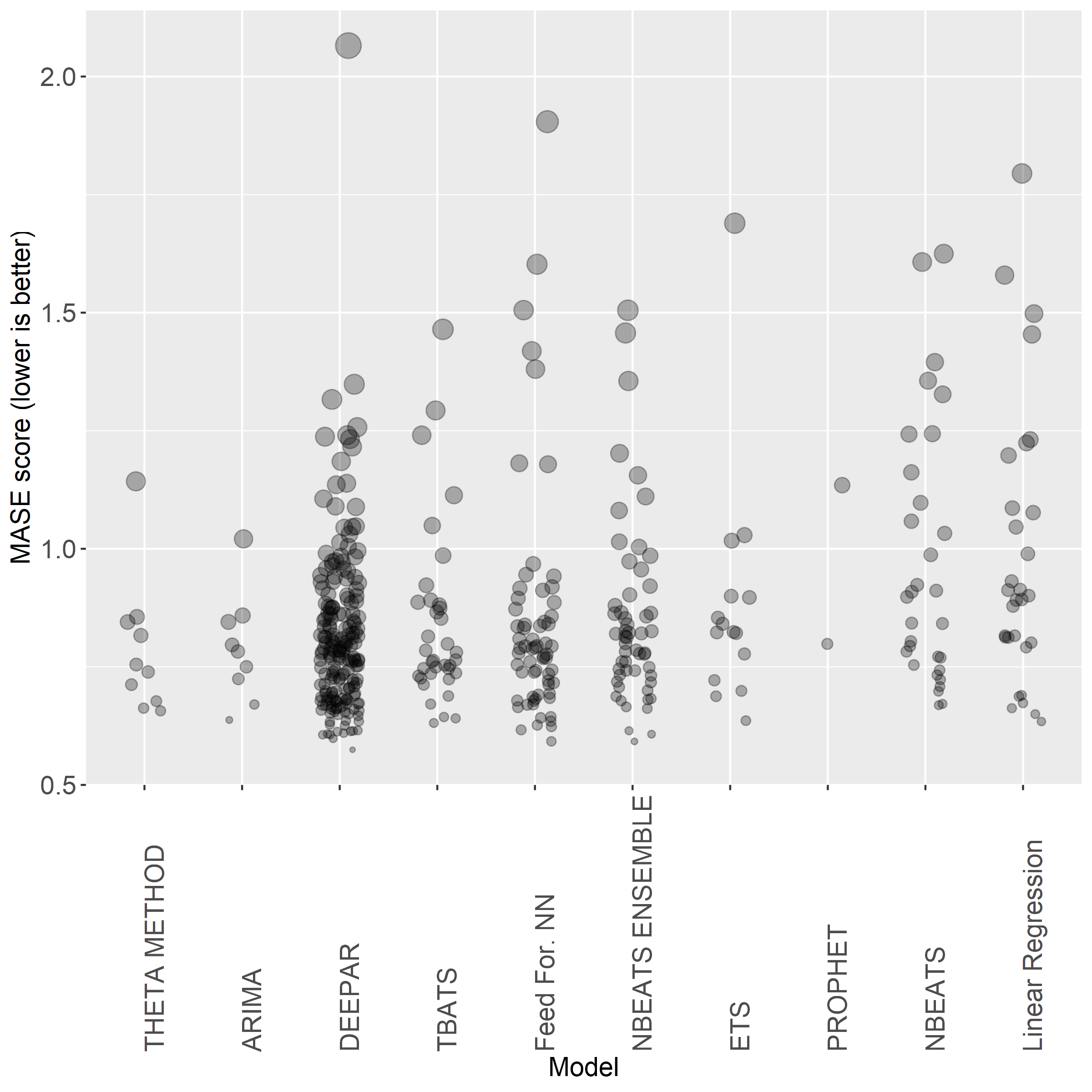
In this plot, each point represents one SKU and the size of the points are determined by how far away that point’s MASE score is from the mean MASE score for that model type. Larger points indicate MASE scores that are well above the mean (very poor accuracy) and smaller points indicate MASE scores well below the mean (very high accuracy). Looking at N-BEATS, you can see there are a number of larger points that are several standard deviations above the mean, which means the forecast was highly inaccurate. These outliers are why the average MASE score differed so much from the median MASE score for these models. By comparison, DeepAR has fewer of these larger points, indicating that it was a more consistent performer.
Conclusions
QueBIT was interested in exploring the efficacy of cutting edge forecasting approaches, like deep learning neural networks, on typical client data where products may have relatively sparse and seemingly random sales patterns. The results presented here indicate that these new approaches, like N-BEATS and DeepAR, warrant further investigation and potential implementation in the forecasting SOP as they were able to strongly outperform forecasts generated by common statistical models. The potential problems I foresee in the implementation of these algorithms is the relatively high computing power required to run them efficiently, which may not be ideal when clients want to use these forecasting tools themselves.