
Building Recurrent Neural Networks in Keras for Time Series Forecasting
Recurrent Neural Network Forecasting with Keras
David Saltzman
The Business Problem
With the proliferation if interest in deep learning across industries, QueBIT wanted to investigate how a deep learning might be used in their forecasting approach for on client data. The dataset we chose covered almost two years worth of data at the daily level, which made it a better candidate for a neural network than sales data, as most sales data to be monthly and insufficient for training a model to outperform a naive forecast.
Data Cleaning
# Import libraries
import pandas as pd
import tensorflow as tf
import numpy as np

# Plotting libraries
import matplotlib.pyplot as plt
import seaborn as sns
sns.set(rc={"figure.dpi":400, 'savefig.dpi':400})

# Import functions that will be needed
from numpy import array
from sklearn.model_selection import train_test_split
from keras.models import Sequential
from keras.layers import Dense
from keras.layers import LSTM
from keras.layers import RNN, SimpleRNN
from keras.preprocessing.sequence import TimeseriesGenerator
from keras.layers import Dropout
from keras.optimizers import Adam
from keras.layers.core import Activation
from keras.callbacks import EarlyStopping
from sklearn.preprocessing import StandardScaler
from sklearn.preprocessing import MinMaxScaler

# Set random seed
np.random.seed(401)
Before preprocessing for the neural network can occur, we need to clean up the data, which is a little messy. I removed the whitespace in some of the cells, removed placeholders that should be NA’s, and other non-standard formatting. There are multiple different time series contained in this dataset, and many of them have missing dates that need to be filled in. For the purposes of testing we narrowed it down to just one SKU that contained very few periods with zero demand.
# Read in data
df = (
  pd.read_csv("rnn_keras_data.csv")
  .rename(columns={'PERIOD_DATE':'DATE',
  'PRODUNIT_ID':'ID',
  'QTY':'QUANTITY'})
  .sort_values(by=['DATE','ID'])
  .astype({'DATE': 'datetime64[ns]'})
)

# Remove whitespace, dashes, and commas from quantity
df['QUANTITY'] = (
  df['QUANTITY']
  .str.strip()
  .replace({'-':'0',',':''},regex=True)
  .astype(int)
)

# Count # of observations for each SKU
print(df['ID'].
  value_counts().
  sort_values(ascending=False))
ID12    650
ID16    644
ID1     644
ID13    642
ID4     642
ID6     642
ID14    637
ID3     636
ID18    623
ID11    617
ID8     611
ID15    611
ID5     609
ID19    597
ID17    596
ID20    574
ID21    574
ID9     539
ID7     516
ID10    495
ID2     433
Name: ID, dtype: int64
In this dataset, missing dates meant that there was no demand on that date, which is meaningful information for our neural network model. In order to fill in those missing dates, I used the package janitor which has a handy function called complete that will allow you to fill out those missing dates by each ID.
# Fill in missing days
import janitor
df = df.complete(
    {'DATE': lambda date: pd.date_range(date.min(), date.max())},
    by = ['ID'],
    fill_value=0,
    sort = True)

# Count # of observations after
print(df['ID'].
  value_counts().
  sort_values(ascending=False))

# Set index
df = df.set_index(['DATE'])

# Subset for testing purposes
df = df[df['ID'] == 'ID1'].reindex()

# Drop ID column as it is no longer needed
df = df.drop('ID',axis=1)
ID1     653
ID19    653
ID11    653
ID12    653
ID13    653
ID14    653
ID15    653
ID18    653
ID16    653
ID20    653
ID21    653
ID3     653
ID4     653
ID5     653
ID6     653
ID8     653
ID17    652
ID7     651
ID10    650
ID9     650
ID2     649
Name: ID, dtype: int64
Much better!
Feature Engineering
The RNN that we are building cannot take dates as an input, and therefore our dataframe column containing the dates needs to be transformed into series that represent each element of the date. This also in turn provides more information to the neural network, which is beneficial as our time series (before feature engineering) was unidimensional.
# Create various temporal features
df_features = (df
                .assign(day = df.index.isocalendar().day)
                .assign(month = df.index.month)
                .assign(day_of_week = df.index.weekday)
                .assign(week_of_year = df.index.isocalendar().week)
                )
Splitting the data
We then split the data using a split of 80% of the data for training, the subsequent 10% of the data for validation, and the final 10% of data is held out to assess the generalization of the model.
# Define the sizes for training, testing, and holdout sets
train_size = 0.8  # 80% of data for training
test_size = 0.2  # 20% of data for testing (will be further split into holdout data )

# Split the data into a training and test set first
train_data, test_data = train_test_split(df_features, test_size=test_size, shuffle=False)

# Then split the remaining data 50/50 (i.e., the "rightmost" portion of the original data) into a test and holdout set
test_data, holdout_data = train_test_split(test_data, test_size=0.5, shuffle=False)

# The resulting data are now split into training, testing, and holdout sets
print("Training data size:", len(train_data))
print("Testing data size:", len(test_data))
print("Holdout data size:", len(holdout_data))
Training data size: 522
Testing data size: 65
Holdout data size: 66
The last step before we can build the model, we need to create a time series generator, which essentially packages our time series data into something that the neural network can use to create batches of input/targets.
# Get number of features and lookback length
n_features = train_data.shape[1]
lookback_length = 5

# create training generator
train_generator = TimeseriesGenerator(
  train_data.values.astype('float32'),
  train_data.values[:,0].reshape((len(train_data.values), 1)).astype('float32'),
  length=lookback_length,
  batch_size=len(train_data)
)

# create test generator
test_generator = TimeseriesGenerator(
  test_data.values.astype('float32'),
  test_data.values[:,0].reshape((len(test_data.values), 1)).astype('float32'),
  length=lookback_length,
  batch_size=1
)

# create holdout generator
hold_generator = TimeseriesGenerator(
  holdout_data.values.astype('float32'),
  holdout_data.values[:,0].reshape((len(holdout_data.values), 1)).astype('float32'),
  length=lookback_length,
  batch_size=1
)
Building the network
Now we get to the fun part, which is assembling the model. Keras allows you to easily assemble complicated models with the .add function, where you define the various layers of your model. A simple recurrent neural network seems like an appropriate place to start for predicting time series, as an RNN keeps a copy of its hidden unit’s previous state and uses it as input to the next iteration. RNN’s have worked well for other types of sequential data, like models of reading, where each word in a sentence builds on the meaning of the previous.
print("timesteps, features:", lookback_length, n_features)

# Initialize model
model = Sequential(name='simpleRNN_Model')

# Add recurrence to model
model.add(SimpleRNN(50, activation='relu', input_shape=(lookback_length, n_features), return_sequences = False))

# Add fully connected layer
model.add(Dense(1, activation='relu'))

# Define optimizer
adam = Adam(learning_rate=0.001)

# Register the custom metric function with the Keras model.
model.compile(loss='mse',optimizer='adam',metrics = ['mse', 'mae'])

# Summarize model we've created
model.summary()
timesteps, features: 5 5
Model: "simpleRNN_Model"

_________________________________________________________________

 Layer (type)                Output Shape              Param #

=================================================================

 simple_rnn (SimpleRNN)      (None, 50)                2800


 dense (Dense)               (None, 1)                 51


=================================================================

Total params: 2,851

Trainable params: 2,851

Non-trainable params: 0

_________________________________________________________________
Fitting the model
It is also a good idea to define an early stopping rule, which is to end model training once validation loss plateaus. If we continue training the model beyond there, we risk venturing into overfitting territory.
# Define early stopping rule
early_stopping = EarlyStopping(monitor='val_loss',
                                patience=5,
                                mode='auto',
                                min_delta=0.1,
                                restore_best_weights=True,
                                verbose=1)

# Fit RNN
score = model.fit(train_generator,
  epochs=1000,
  validation_data=test_generator,
  callbacks=[early_stopping],
  verbose=0)
Restoring model weights from the end of the best epoch: 176.

Epoch 181: early stopping
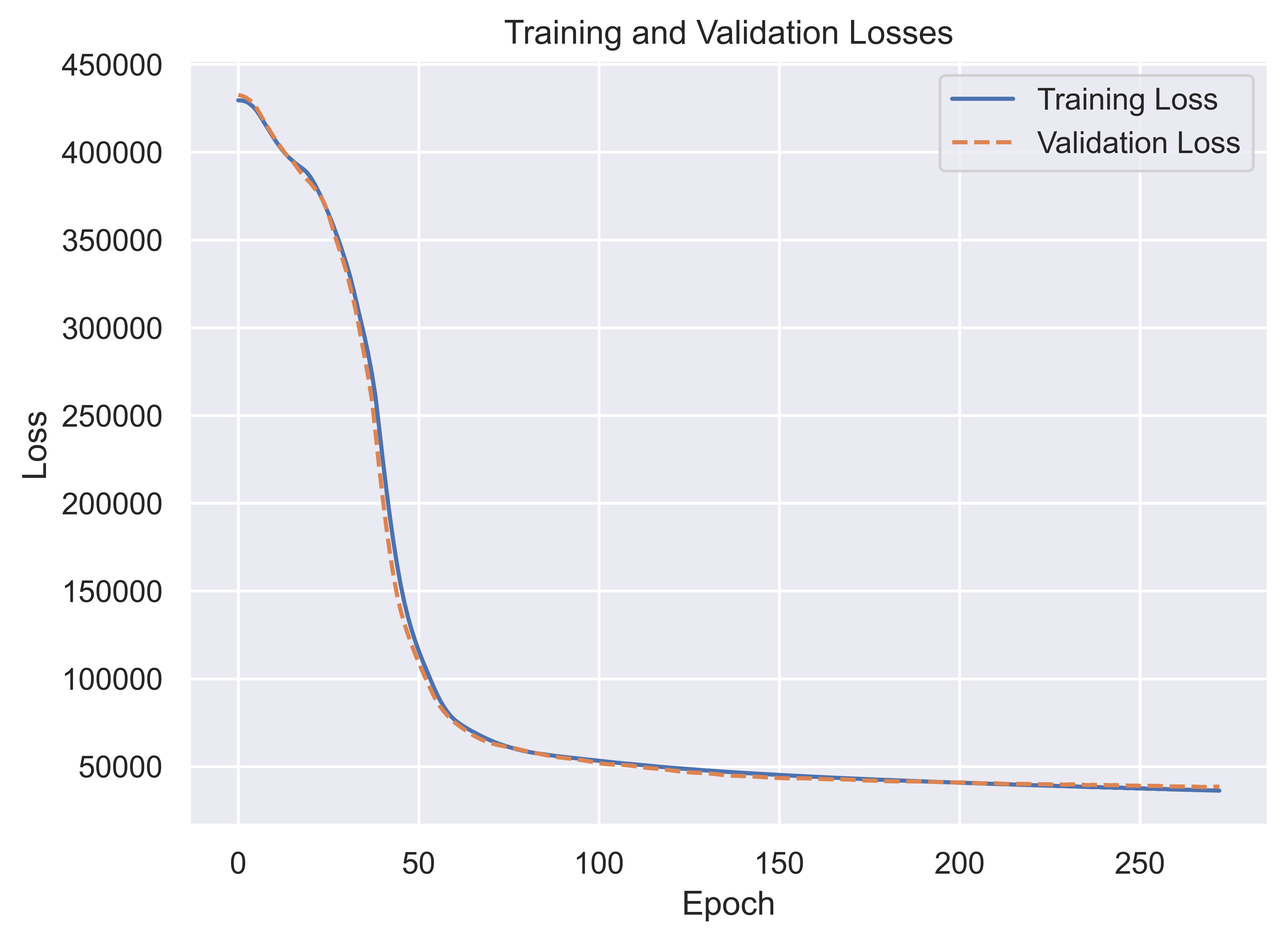
Now that the model has been fit, we can plot the validation and training loss, which we can see plateaus and then stops way earlier than the 1,000 epochs we set for the model to potentially iterate through.
Next we can look at the accuracy of the model on the validation data:
# Create list to put results in
results_list = []

# Loop through actuals and get predictions from model
for i in range(len(hold_generator)):
    x, y = hold_generator[i]
    x_input = array(x).reshape((1, lookback_length, n_features))
    yhat = model.predict(x_input, verbose=0)
    results_list.append({'Actual': y[0][0], 'Prediction':yhat[0][0]})

# Convert to dataframe
df_result = pd.DataFrame(results_list)

# Calculate MASE
from sktime.performance_metrics.forecasting import MeanAbsoluteScaledError
mase = MeanAbsoluteScaledError()

simple_rnn_mase = round(mase(
y_true=df_result['Actual'],
y_pred=df_result['Prediction'],
y_train=train_data['QUANTITY']),2
)

print("MASE Score:",simple_rnn_mase)
MASE Score: 1.13
Our simple RNN network performed worse than a naive forecast, but not very far off, which is promising. For difficult to predict time series like this one, often you will not get a model that outperforms a naive forecast, so this result is not unexpected. Next we can look at a plot of the predictions against the actuals:
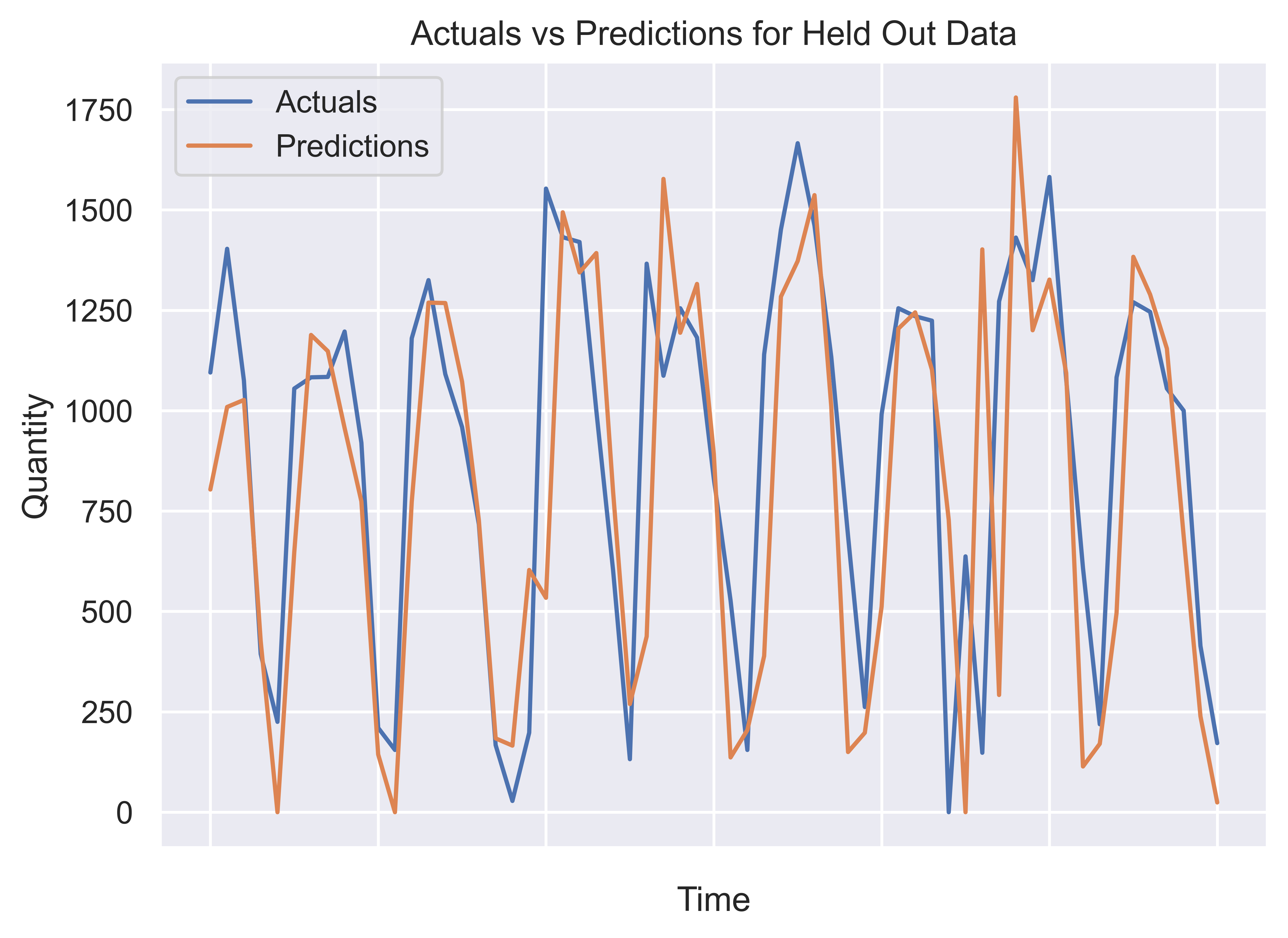
The RNN is approximating the general shape of the held out data most of the time, which is promising. While there is a lot more tuning of this model that could be done, this is a decent baseline already!
Using an LSTM instead of Simple RNN
While RNN’s are a powerful way to model sequential data like a time series, a Long Short-Term Memory (LSTM) is a newer approach to neural networks that can track longer term dependencies more effectively than a RNN. We can build an LSTM model and compare its performance to our simple RNN. Below I build a deep LSTM network by stacking three LSTM networks.
# Initialize model
model2 = Sequential(name="LSTM_Model")

# Add three LSTM layers
model2.add(LSTM(100, activation='relu', input_shape=(lookback_length, n_features), return_sequences = True))
model2.add(LSTM(50, activation='relu', input_shape=(lookback_length, n_features), return_sequences = True))
model2.add(LSTM(25,activation='relu'))

# Add fully connected layer
model2.add(Dense(1, activation='relu'))

# Define optimizer
adam = Adam(learning_rate=0.001)

# Register the custom metric function with the Keras model.
model2.compile(loss='mse',optimizer='adam',metrics = ['mse', 'mae'])

# Summarize model we've created
model2.summary()
Model: "LSTM_Model"

_________________________________________________________________

 Layer (type)                Output Shape              Param #

=================================================================

 lstm (LSTM)                 (None, 5, 100)            42400


 lstm_1 (LSTM)               (None, 5, 50)             30200


 lstm_2 (LSTM)               (None, 25)                7600


 dense_1 (Dense)             (None, 1)                 26


=================================================================

Total params: 80,226

Trainable params: 80,226

Non-trainable params: 0

_________________________________________________________________
In this case, we have created a much more complicated model, as the number of parameters is several orders of magnitude greater than our simple RNN. Fitting the model will tell us if this increase in complexity is worth it:
# Fit model
score2 = model2.fit(train_generator,
  epochs=1000,
  validation_data=test_generator,
  callbacks=[early_stopping],
  verbose=0)

# Create list to put results in
results_list2 = []

# Loop through actuals and get predictions from model
for i in range(len(hold_generator)):
    x, y = hold_generator[i]
    x_input = array(x).reshape((1, lookback_length, n_features))
    yhat = model2.predict(x_input, verbose=0)
    results_list2.append({'Actual': y[0][0], 'Prediction':yhat[0][0]})

# Convert to dataframe
df_result2 = pd.DataFrame(results_list2)

# Calculate MASE
from sktime.performance_metrics.forecasting import MeanAbsoluteScaledError

mase = MeanAbsoluteScaledError()

print("MASE score:", round(mase(y_true=df_result2[['Actual']],y_pred=df_result2[['Prediction']].astype('float32'),y_train=train_data['QUANTITY']),2))
Restoring model weights from the end of the best epoch: 51.

Epoch 56: early stopping

MASE score: 1.48
The MASE score on the held out data for the deep LSTM model is worse than that of the simple RNN, which is not entirely unexpected. More tuning could be performed to improve the performance of this model, but it’s also possible that there just isn’t sufficient training data to warrant a model this complicated.
Ultimately, we concluded that deep learning is a very important domain to monitor as it becomes more and more accurate at predicting time series data, but in the near future it is unlikely most clients will have sufficient data to train a model that will outperform conventional statistical analyses.